Why does the degrees of freedom in Linear Regression equal n-p?

If we run linear regression in R, then we will see a term in the report “degrees of freedom” and that value equals n-p where n is the number of observations (data points) and p is the number of parameters (including intercept).

But what does it mean? How is it useful?

Short Answer: the degree of freedom represents the number of “free” or independent $N(0,1)^2$ in the residuals from linear regression. The following three parts will explain this further.

1. Measure $\sigma^2$

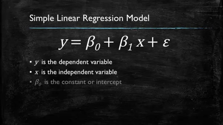
Under the Gauss-Markov model, which states $y_i = x_i^{T}\beta+\epsilon_i$ where $\epsilon$ are iid errors centered at zero with variance $\sigma$. Here, $x_i$ and $\beta$ are all assumed determined. $\epsilon_i$ are the randomness here, which cause y to be random.

With the widely known $(X^TX)^{-1}X^TY$ formula, one can derive the BLUE estimator $\hat{\beta}$ for $\beta$ and obtain estimated residual $\hat{\epsilon}$. Then, how can we estimate $\sigma$? We have RSS, which is the residual sum of squares but what’s next?

A short answer is: $E(\frac{RSS}{n-p}) = \sigma^2$. Here, the denominator is the degree of freedom. Proof follows from the fact that $cov(\hat{\epsilon})=\sigma^2 (I_n-H)$ , where H is the projection matrix and error term centers at zero.

To make the proof easier, let us further assume error terms follow normality. Then, $RSS=\sum_{i=1}^{N}\hat{\epsilon^2}$ is similar to a chi-square distribution. Note, chi-square distribution with l degree of freedom means sum of l standard normal’s square.

But they are not identically the same. Actually, $\frac{RSS}{\sigma^2} \sim \chi_{n-p}$ because the trace of (1-H) is n-p. This is because the eigenvalues of (1-H) is n-p and that is exactly the number of independent normal variables in the residual. $E(\chi^2_{n-p})=n-p$ so $E(\frac{RSS}{n-p}) = \sigma^2$

2. Hypothesis Testing for $\hat{\beta}$

$$\frac{\hat{\beta} - \beta}{\sqrt{\hat{\sigma^2}}(X^TX)^{-1}} \sim t_{n-p}$$

n-p is also the degree of freedom of t distribution for testing whether $\beta$ is zero. Note, t distribution $t_{n-p}=\frac{N(0,1)}{\sqrt{\chi^2_{n-p}/(n-p)}}$. The n-p comes from the same chi-square distribution as we mentioned above.

But here, the assumption is that error term follows homoscedasticity. How do we estimate the standard error for $\hat{\beta}$ under heteroscedasticity? It will be in the future posts about EHW and WLS.

3. Connection to 1-sample t-test

Let us first assume that we have shifted the Y with a null hypothesized mean $y_i = y_i - Y_0$ for all i. Then, if the linear model is $Y \sim 1$, which only includes the interception term, then $\beta = \bar{Y}$, the sample average of Y. The RSS/(n-1) will be exactly the same as the sample variance of Y. We can notice that this is another reason for minus 1 in the denominator for computing sample variance. By part II, sample mean over sqrt of sample variance follows a t-distribution with df n-1.

4. Connection to 2-sample t-test

Let us assume that the linear model is $Y \sim 1 + X$, which includes the interception term and a binary variable X only takes 0 for 1. Moreover, X is 0 for control group and X is 1 for treatment group. We want to test whether the average treatment effect or diff-in-means significant enough. If we run the regression, the coefficient for X will be the diff-in-means estimator (difference between two sample mean). The standard error of beta will be the same as that of a 2-sample t-test if you algebraically solve for it by the equation above. Furthermore, the degree of freedom will be n-2 since p equal to 2 in this case.